Calculating size distribution
of powder particles using ImageJ

Motivation

Our group in Prague received samples of tiny dielectric resonators made of TiO2 spheres with diameter of 0.03 to 0.1 mm. (For more details, see Ref. 1) At a first glance they look like white powder. The resonant frequency was measured to lie between 400 and 1200 GHz using time-domain terahertz spectroscopy. However the resonance was quite weak and broadband, which was expected to be mainly a result of uneven sizes of the spheres.

To measure a reliable size distribution of the particles, I took several photos of one sparse layer of the particles with a microscope. Then I used ImageJ to automatically recognize individual spheres using a macro. Finally I processed the data to plot nice histograms using Python+Scipy+Matplotlib. (Unfortunately I did not find any more convenient way to do this without ImageJ. There is probably a bug in the watershed function in Scikits-image, which forced me to launch ImageJ instead of python module.)

Images

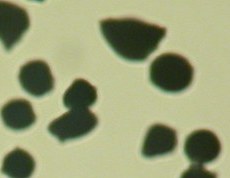
1. Cropped photo of particles
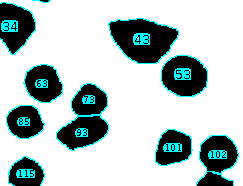
2. Particles separated and recognized by ImageJ
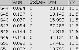
3. Table of particles and their parameters in ImageJ
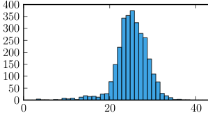
4. Histogram from Python+Matplotlib showing the average of 25 microns and deviation of 4 microns for the shorter ellipse axis

Requirements

• For image processing and particle recognition: ImageJ (or FIJI, which is just ImageJ)
• I used Ubuntu Linux, but other operating systems should work as well, as all used software is multiplatform.

Python script for particle counting and statistical analysis

The following python script uses an ImageJ macro similar to the one in Appendix, and it processes its output.

Do not forget to modify the dir_prefix and dir_names variables to point to your directories with the images! After all, you will probably want to read it and modify it to your needs.

#-*- coding: utf-8 -*-
"""
I wrote a macro for the ImageJ program to automatically measure particle shapes on 
a photograph. The particle sizes are then processed to plot a size distribution 
of the powder. The process is fully automatic, allowing many images or samples to 
be processed in a batch.

This program runs ImageJ and plots the histogram.

Requirements: ImageJ, matplotlib. Tested on Ubuntu 11.10 with Python 2.7.

See details at http://fzu.cz/~dominecf/misc/imagej_particles.html

Copyright (c) 2012-01-08 Filip Dominec 
This software is free as speech after five beers. Published under BSD license.
"""


import sys, traceback, subprocess, os

import matplotlib
import matplotlib.pyplot as plt
import scipy.integrate
import scipy.interpolate
matplotlib.rc('text', usetex=True)
matplotlib.rc('font',**{'family':'serif','serif':['Computer Modern Roman, Times, Palatino, New Century Schoolbook, Bookman']})
matplotlib.rc('text.latex',unicode=True)
colors = ("#BB3300", "#8800DD", "#2222FF", "#0088DD", "#00AA00", "#AA8800",
                       "#661100", "#440077", "#000088", "#003366", "#004400", "#554400")
plt.figure(figsize=(8,10))

path_to_imagej_macro="/tmp/particle_counting.imj"
dir_prefix = "powder_stats/"
#dir_names = ["input"]
dir_names = [
    "sub38",
    "38-40",
    "40-50",
    "53",
    "100",
    ]   

def prepare_macro_file(path_to_imagej_macro):
    """ Writes an ImageJ macro to the disk, to be used later in a batch. """
    ImageJ_macro =  """

        open(getArgument());
        run("8-bit");
        run("Enhance Contrast", "saturated=.4 normalize");
        run("Threshold", "method=Default white");
        run("Watershed");
        run("Set Measurements...", "area mean center perimeter fit shape display redirect=None decimal=5");
        run("Set Scale...", "distance=1324 known=1000 pixel=1 unit=um global");
        run("Analyze Particles...", "size=1e1-1e6 circularity=0.10-1.00 show=[Overlay Outlines] display exclude clear include");
        close()

        """
    macro = open(path_to_imagej_macro, "w")
    macro.write(ImageJ_macro)
    macro.close()

def resolve_particles(file_name, path_to_imagej_macro):
    """ Invokes ImageJ to process the image and to save the statistics. Returns two scipy.arrays of major and minor axes of the ellipses. """
    
    ## To run non-interactively in batch mode, ImageJ has to read a macro from disk.
    ## The third parameter is the image to be processed.
    command = "imagej -b '" + path_to_imagej_macro + "' '" + file_name + "'"
    p = subprocess.Popen(command, shell=True, stderr=subprocess.PIPE, stdout=subprocess.PIPE)
    out = p.stdout.read().strip()


    ## The format of output string is now as follows:
    #     Label            Area    Mea    XM        YM        Perim.    Major    Minor    Angle        Circ.    AR        Round    Solidity
    #1    DSCN2117.JPG    0.00066    255    0.76635    0.01473    0.09917    0.03240    0.02603    168.37377    0.84632    1.24490    0.80328    0.95125
    major = scipy.array([])
    minor = scipy.array([])
    for line in out.split("\n")[4:]:        # skip initial header+garbage
        try:
            major = scipy.append(major, float(line.split()[7]))
            minor = scipy.append(minor, float(line.split()[8]))
        except:
            pass
    return major, minor


prepare_macro_file(path_to_imagej_macro)        # go through all subdirectories (which are different samples)
for n, dir_name in enumerate(dir_names):
    ## Init statistics for one sample
    print "Entering directory: " + dir_name
    major = scipy.array([])
    minor = scipy.array([])

    ## Create vertically aligned graphs
    plt.subplot(len(dir_names)*100 + 10 + n + 1)

    ## Use the cached results if available, otherwise run ImageJ to find the particles
    stats_cache_dir_name = "stats_cache/"
    stats_cache_file_name = stats_cache_dir_name+dir_name+".csv"
    if os.path.exists(stats_cache_file_name):
        major, minor = scipy.loadtxt(stats_cache_file_name)
    else:
        ## Go through all files in directory (which all describe one sample)
        for file_name in os.listdir(dir_prefix+dir_name):
            file_name_w_path = dir_prefix+dir_name+"/"+file_name
            print "\tProcessing image ", file_name_w_path + "... ",
            major_new, minor_new = resolve_particles(file_name_w_path, path_to_imagej_macro)

            ## Add the statistics of one photo to the cumulative statistics
            major = scipy.append(major, major_new)
            minor = scipy.append(minor, minor_new)
            print "Added " + `len(major_new)` + " particles"

        ## Save the results
        if not os.path.exists(stats_cache_dir_name): os.makedirs(stats_cache_dir_name)
        scipy.savetxt(stats_cache_file_name, (major,minor))


    ## Print out statistics of major and minor axes
    major_average = sum(major)/len(major)
    major_sigma = sum((major - major_average)**2/len(major))**.5
    minor_average = sum(minor)/len(minor)
    minor_sigma = sum((minor - minor_average)**2/len(minor))**.5

    print "\tTotal particles fitted with ellipse: ", len(major)
    print "\tMajor avg, sigma: ", major_average, major_sigma
    print "\tMinor avg, sigma: ", minor_average, minor_sigma

    ## Plot the histogram of the data
    n, bins, patches = plt.hist(major, bins=100, range=(0, 99), normed=False, facecolor=colors[n+1], alpha=0.75, linewidth=.8)
    plt.annotate("\\noindent Sample name: "+dir_name+"\\\\ (mean = $%.1f$, $\\sigma=%.1f$)" % (major_average, major_sigma), 
            xy=(.97, .90),  xycoords='axes fraction', 
            horizontalalignment='right', verticalalignment='top')
    #plt.grid(True)

## Finish the graph
plt.xlabel(u'Longer ellipse axis [$\\mu$m]')
plt.savefig("powder_stats.pdf")

Appendix: ImageJ macro for particle counting

If you do not want to use Python, you can get the particle statistics for a directory using bare ImageJ macro. Save this file to "/tmp/particle_counting.imj":

setBatchMode(true); 
function action(input, output, filename) {
 		open(input + filename);
		run("8-bit");
		run("Enhance Contrast", "saturated=4 normalize");
		run("Threshold", "method=Default white");
 		run("Watershed");
 		run("Set Measurements...", "area mean center perimeter fit shape display redirect=None decimal=5");
 		run("Set Scale...", "distance=1324 known=1 pixel=1 unit=mm global");
 		run("Analyze Particles...", "size=.00-1 circularity=0.10-1.00 show=[Overlay Outlines] display exclude clear include");
 		saveAs("PNG", output+filename);

		saveAs("Results", output+filename+"results.csv" );
		run("Clear Results");

 		close();
}
input = "/tmp/fiji/input/"; 
output = "/tmp/fiji/output/";
list = getFileList(input); 
for (i = 0; i < list.length; i++)         
		action(input, output, list[i]);
setBatchMode(false);

I hope that all the commands are self-explanatory. You may use them in interactive session of ImageJ to see what they do.

Generally, this macro goes through all images in given directory. Each image gets thresholded to white and black at 50%-level between background and particle color; this prevents the possible blur of the photograph from altering the average particle size. All touching particles should be split by the watershed algorithm. Then ImageJ resolves all particles. It saves the particle outlines to a new image and the particle parameters to a CSV file. These two output files are named similarly as the input file.

The image size was calibrated using one photograph of a ruler. There is an option in ImageJ directly for this calibration. You will want to change the corresponding command before running the batch.

(Tip: To find out what all the measurement values mean, you may look at here.)

References

1. H. Němec, C. Kadlec, F. Kadlec, P. Kužel, R. Yahiaoui, U-C. Chung, C. Elissalde, M. Maglione and P. Mounaix, "Resonant magnetic response of TiO2 microspheres at terahertz frequencies," Appl. Phys. Lett (submitted).